Attention Is All You Need
이번엔 오늘날의 NLP계의 표준이 된 Transformer를 제안한 논문인 Attenion Is All You Need에 대해서 리뷰해보고자 한다. 대략적인 내용은 이미 알고 있었지만, 디테일한 부분도 살펴보고자 한다.
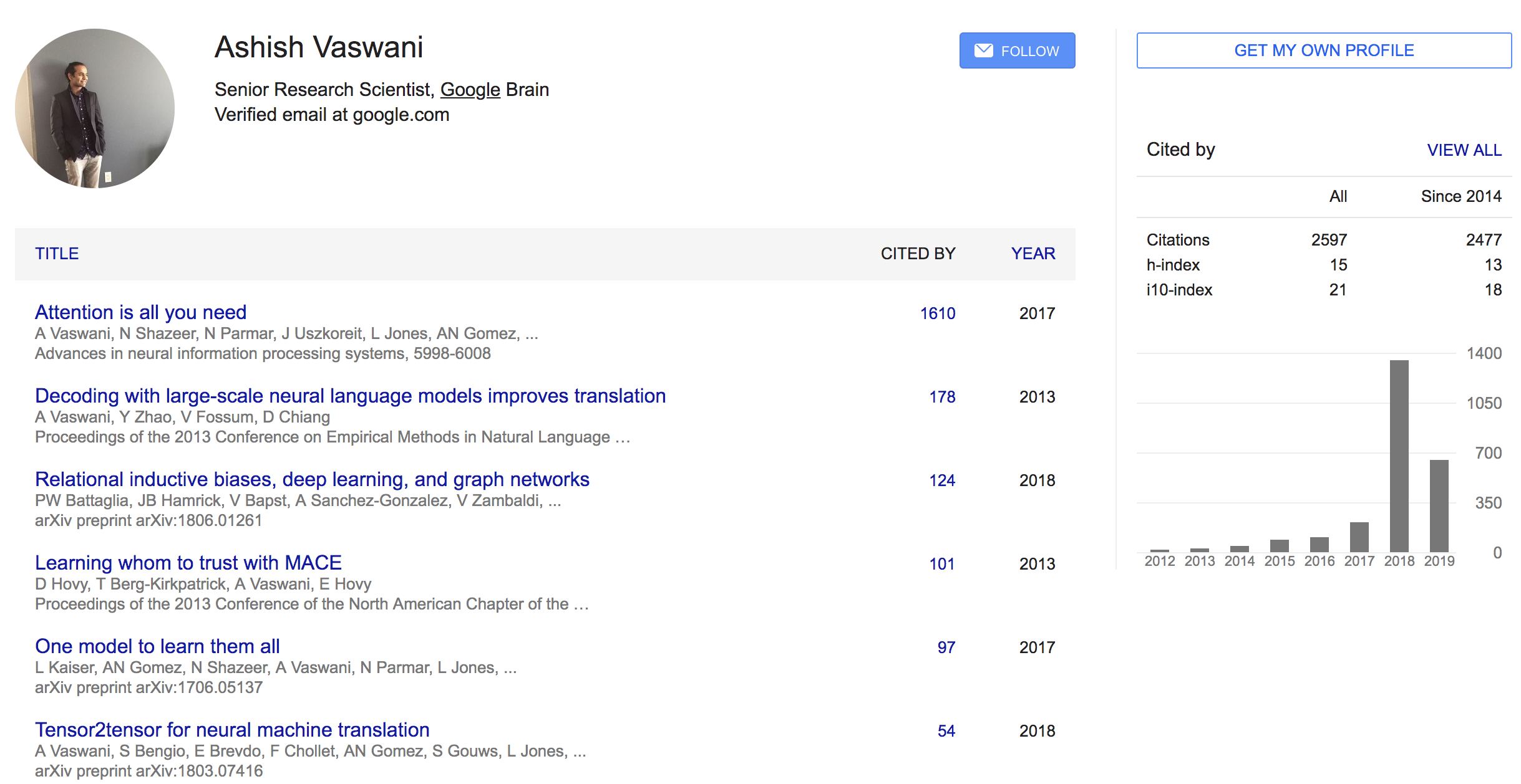
Author
- 저자: Ashish Vaswani, 외 7명 (Google Brain)
구글브레인..wow- NIPS 2017 accepted
Who is an Author?
 {: height=”50%” width=”50%”}
느낀점
- Multi-Head-Attention을 빠르게 구현하기 위해 Matrix 연산으로 처리하되, Embedding Tensor를 쪼갠 후 합치는게 아닌 reshape & transpose operator로 shape을 변경 후 한꺼번에 행렬곱으로 계산해서 다시 reshape 함으로써 병렬처리가 가능하게끔 구현하는게 인상적이었음
- 행렬곱할 때 weight 와 곱하는건 weight variable 생성 후 MatMul 하는게 아니라 그냥 다 Dense로 처리하는게 구현 팁이구나 느꼈음
- 요약: 쪼갠다음에 weight 선언 후 매트릭스 곱? No! -> 쪼갠 다음에 Dense! -> 쪼개면 for loop 때문에 병렬처리 안되잖아! -> 다 계산후에 쪼개자!
- Attention만 구현하면 얼추 끝날 줄 알았는데 Masking 지분이 70~80%였음
- Masking은 logical 연산 (boolean)으로 padding 체크해서 하는게 일반적임
- Masking은 input에도 해주고 loss에도 해줌
- 마스킹 적용할땐 broadcasting 기법을 써서 하는게 일반적임
- 아래의 두 경우 모두 가능함
- ex) (40, 5, 10, 10) + (40, 1, 1, 10) == (batch, head, seq, seq)
- ex) (40, 5, 10, 10) + (40, 1, 10, 10) == (batch, head, seq, seq)
Abstract
- 대부분의 sequence 모델들은 encoder-decoder 프레임워크를 포함해서, 복잡한 RNN이나 CNN이었음
- 최고의 성능을 내는 모델 역시 encoder-decoder 프레임워크안에서 동작하지만, Attention mechansim으로 모델링했음
- 본 논문에서는 Transformer라는 오직 Attention mechansim에만 기초한 simple neural architecture를 제안함
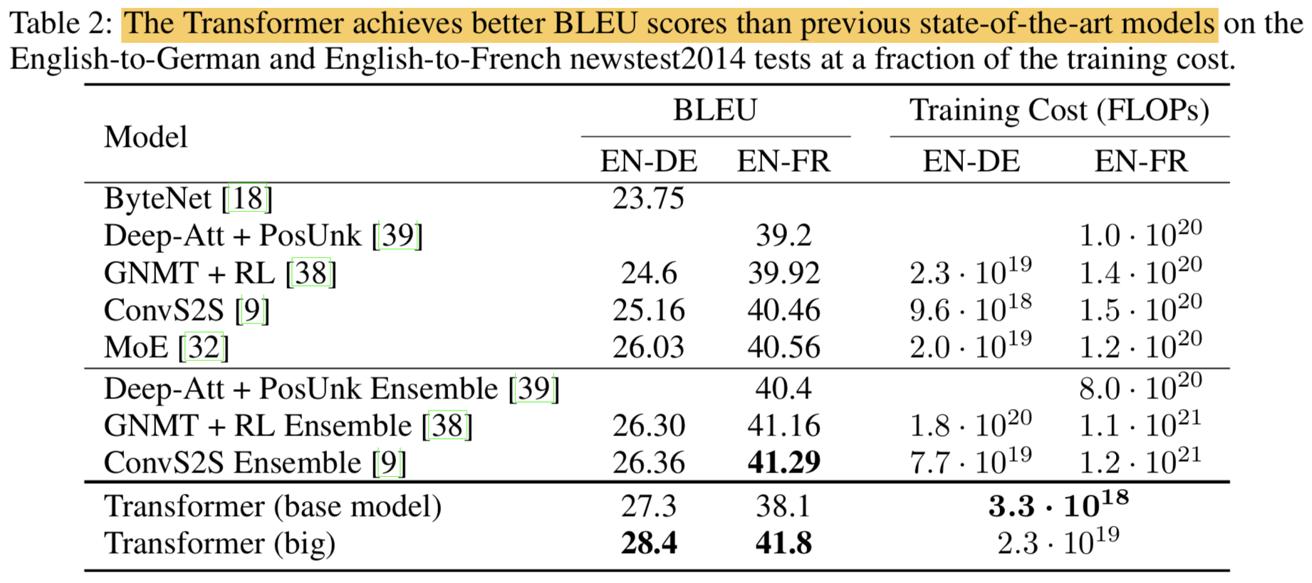
RNN이나 CNN따위 없음..- 2개의 machine translation task에 대해서 실험했고, 병렬화도 잘되고 학습시간도 짧으면서 퀄리티도 우월함을 확인함
- WMT 2014 English-to-German translation task에서 28.4 BLEU를 기록함 (다른 모델보다 2 BLEU 정도 높음)
- WMT 2014 English-to-French translation task에서는 41.8 BLEU로 SOTA 기록함 (8 GPUs로 3.5days 걸림)
- 다른 Task에서도 Generalize 잘됨
1. Introduction
- RNN, LSTM, GRU 등은 sequence modeling (language modeling, machine translation)에서 SOTA를 기록해왔음
- 대부분 노력들은 recurrent language model, encoder-decoder 구조 내에서 이뤄졌음
- RNN 계열의 모델들은 input, output의 sequence 내에서 position을 따라 계산되는 특징이 있는데, 이는 병렬처리를 막고, 시퀀스 길이가 길어지면 문제가 생기는등의 여러가지 이슈가 있음
- Attention mechansim은 sequence 내에서 거리에 상관 없이 dependency modeling이 가능하기 때문에 sequence modeling을 정복할 수 있음
- 기존엔 RNN 계열에 Attention이 적용되었는데, 본 논문에서 제안하는 Transformer는 recurrence 방식을 피하고, 대신 전적으로 attention mechanism에만 의지해서 input, output 사이의 global dependency를 고려하고자 함
- Transformer는 병렬처리도 잘되고, 성능도 SOTA임 (학습시간은 12시간 걸렸음 with 8 P100 GPUs)
2. Background
- Sequential computation 문제를 해결하기 위해
the Extended Neural GPU,ByteNet,ConvS2S등 CNN을 hidden representations을 병렬처리로 계산하기 위한 basic building block으로 사용하려는 연구들이 있었음 - 위의 연구들은 dependency를 고려하려는 관점에서 볼 때, distance에 대해서 linear (ConvS2S), 혹은 logarithm (ByteNet) 한 고려가 가능했음
- 하지만 position의 거리에 따른 dependency를 학습하는건 더 어렵게 만들었음 (
이 부분은 잘 이해가 안가네.. 음 그 이전 모델보다는 더 잘되는거 아닌가? 지적하는 근거가 뭐지..) - Transformer에서는 constant 레벨까지 operation 숫자를 줄일 수 있음(
N개에 대한 dependency있지만 병렬처리가 가능해서 그런듯..?) - Self-Attention (다른 말로, intra-attention)은 한 시퀀스 내에서 서로 다른 position들의 관계 representation을 계산하기 위한 attention mechanism임
- Self-attention은 이미 여러 task에서 성공했음 (reading comprehension, abstractive summarization, textual entailment, learning task-independent sentence representations)
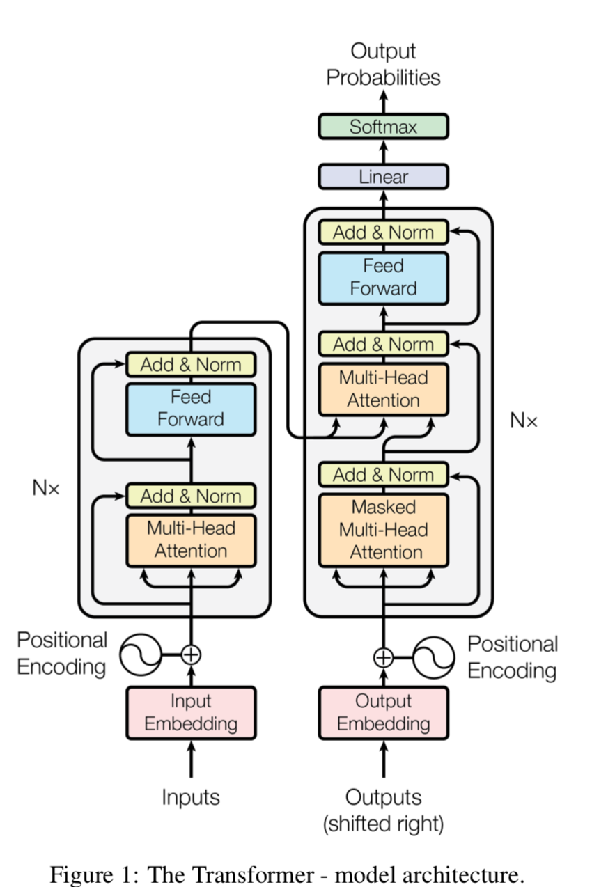
3. Model Architecture
- 대부분 경쟁력있는 sequence transduction model은 encoder-decoder 형태임
- encoder는 input sequence of symbol representations (x1,…,xn)을 continuous representations (z1, …, zn)로 맵핑하는 역할을 함
- decoder는 주어진 z로 부터 output sequence (y1, …, ym)를 생성함
- 각 스텝에서 모델은 auto-regressive함(previously generated symbol을 addtional input으로 사용)
 {: height=”50%” width=”50%”}
3.1. Encoder and Decoder Stacks
- Encoder
- 인코더는 N = 6 개의 identical layer의 스택으로 이루어져있음
- 각 layer는 두 개의 sub-layer로 이루어져있음
- 첫번째는 multi-head self-attention mechansim
- 두번째는 position-wise fully connected feed-forward network
1
2
3
4
5
6
7
8
def sub_layer(self, x, training=False, padding_mask=None):
out_1, attention_weight = self.mha(x, K = x, V = x, mask=padding_mask, flag="encoder_mask")
out_1 = self.dropout1(out_1, training=training)
out_2 = self.layer_norm_1(out_1 + x)
out_3 = self.position_wise_fc(out_2)
out_3 = self.dropout2(out_3, training=training)
out_4 = self.layer_norm_2(out_2 + out_3)
return out_4, attention_weight
- 두 개의 레이어에 각각 residual connection & layer normalization을 적용함
- 각 sub-layer의 output은 LayerNorm(x + Sublayer(x)) 형태임
- layerNorm은
tf.keras.layers.LayerNormalizationAPI로 쉽게 구현 가능함 - Hidden units들에 대해 Norm을 계산하기 때문에 Batch Norm과 다르다고함 (추가로 공부 필요)
- layerNorm은
where Sublayer(x) is the function implemented by the sub-layer itself1
2
3
4for i in range(self.layer_num):
x, attention_block1, attention_block2 = self.sub_layer(x, encoder_ouput, training, look_ahead_mask, padding_mask)
attention_weights['decoder_layer{}_block1'.format(i + 1)] = attention_block1
attention_weights['decoder_layer{}_block2'.format(i + 1)] = attention_block2- residual connection을 하기 위해서 모델에 있는 모든 sub-layer는(embedding layer까지 포함) output의 dimension dmodel = 512 로 셋팅함
- Decoder
- 디코더 또한 N = 6 개의 identical layer의 스택으로 이루어져있음
- 디코더에는 2개가 아닌 3개의 sub-layer로 구성됨
- 첫째는 Masked Multi-Head self-Attention 임. 입력 포지션 상에서 이어서 나오는 것들을 마스킹해버려서 position i 를 예측할때 known outputs at position less than i 만 사용 가능하게 함
- 두번째는 Multi-Head Attention임 얘는 encoder의 output에 적용됨
- 세번째는 Feed Forward Network임
- 결국 첫번째 sub-layer가 좀 특이한거고 두번째 sub-layer의 인풋에 encoder의 output이 들어가는 게 차이임
1
2
3
4
5
6
7
8
9
10
11def sub_layer(self, x, encoder_ouput, training=False, look_ahead_mask=None, padding_mask=None):
out_1, attention_weight_lah_mha_in_decoder = self.look_ahead_mha(x, K = x, V = x, mask = look_ahead_mask, flag="look_ahead_mask")
out_1 = self.dropout1(out_1, training=training)
out_2 = self.layer_norm_1(out_1 + x)
out_3, attention_weight_pad_mha_in_decoder = self.mha(out_2, K = encoder_ouput, V = encoder_ouput, mask = padding_mask, flag="padding_mask")
out_3 = self.dropout2(out_3, training=training)
out_4 = self.layer_norm_2(out_3 + out_2)
out_5 = self.position_wise_fc(out_4)
out_6 = self.layer_norm_3(out_4 + out_5)
return out_6, attention_weight_lah_mha_in_decoder, attention_weight_pad_mha_in_decoder
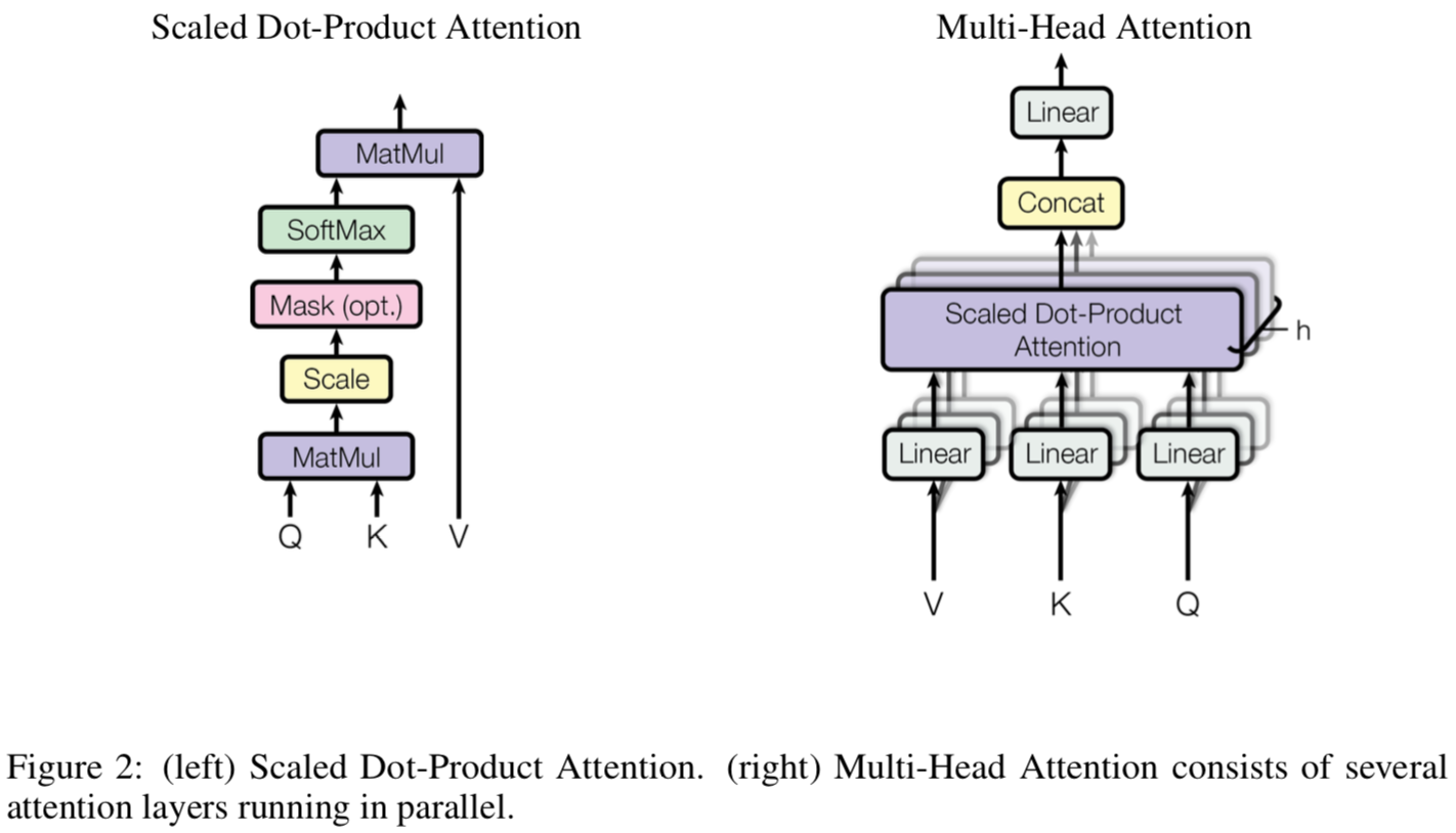
3.2. Attention
- Attention function은 query와 key-value pair를 output에 매핑하는것으로 설명 가능함
- 여기서 말하는 query, key, value는 모두 vector를 의미함
- output은 value에 대한 weighted sum으로 계산되는데, 이 value에 할당되는 이 weight는 query에 대응되는 key의 compatibility function에 의해 계산됨
- 결과적으로 Query와 Key의 유사도로 weight 결정되고 이걸 적용하겠다는 것임
- key와 value는 같은 벡터를 의미함
- key는 weight 뽑는 용
- value는 weight를 적용할때 실제 곱해지는 용
 {: height=”50%” width=”50%”}
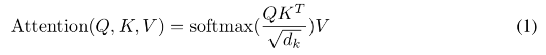
3.2.1. Scaled Dot-Product Attention
- 본 논문에서 쓰는 어텐션을 “Scaled Dot-Product Attention”이라 칭함
- input은 queries, keys 라고 보면 되고 key의 dimension은 dk value의 dimension은 dv 임
- 먼저 query와 모든 key에 대해서 dot product를 계산함
- 계산한 값에 대해서 각각에 대해 $\sqrt{d_k}$로 나눠줌 (여기서 Scaled라는 단어가 나온게 아닌가 싶음, 근데 왜 $\sqrt{d_k}$로 나눠줄까? 다른것들도 어차피 똑같이 나눠주면 softmax에 영향 없을거같은데 음.. $e^x$의 input 스케일에 따라 값이 차이나서 그런건가..)
- softmax function으로 value에 적용할 weight를 얻음
- 실제로 쓸 땐, A set of queries에 대한 Attention은 동시에 계산하기 때문에 Matrix 형태로 사용함
 {: height=”50%” width=”50%”}
- 많이 쓰이는 Attention은 주로 additive attention & dot-product attention인데 본 논문에서 쓴건 dot-product쪽임, 1/$\sqrt{d_k}$로 스케일링 해줬다는 차이가 있긴 함
- 이론적으론 둘 다 복잡도는 비슷하나, dot-product attention이 훨씬 빠르고 space-efficient한 이유는 highly optimized matrix multiplication code로 구현되어있기 때문임
- 1/$\sqrt{d_k}$로 스케일링한 이유는 (
이제 나오네) $d_k$ 값이 클 경우 dot product 값이 커지고, 이는 softmax function이 small gradients를 갖게 만드는 것이 아닌지 의심이 되었고 이러한 효과를 막기 위해 스케일링 한 것임 (얼추 맞았다) ($d_k$가 작은 경우 스케일링을 해주지 않으면 additive attention 성능이 더 좋다고 함)1
2
3
4
5
6
7
8
9
10
11
12
13def scaled_dot_product_attention(self, Q, K, V, mask=None, flag=None):
matmul_qk = tf.matmul(Q, K, transpose_b=True) # (batch, head_num, seq, split_embed_dim) * (batch, head_num, split_embed_dim, seq) = (batch, head_num, seq, seq)
dk = tf.cast(tf.shape(K)[-1], tf.float32) # dk dim
scaled_dot_product_qk = matmul_qk / tf.math.sqrt(dk)
if mask is not None:
minus_infinity = -1e9
scaled_dot_product_qk += mask * minus_infinity # broadcasting, masking에서 seq은 마지막자리
# mask와 scaled_dot_product_qk의 차원은 다르지만, 마지막 차원이 같기 때문에 broadcasting이 가능함
attention_weight = tf.nn.softmax(scaled_dot_product_qk, axis=-1)
scaled_attention_output = tf.matmul(attention_weight, V) # (batch, head_num, seq, seq) * (batch, head_num, seq, split_embed_dim) = (batch, head_num, seq, split_embed_dim)
return scaled_attention_output, attention_weight
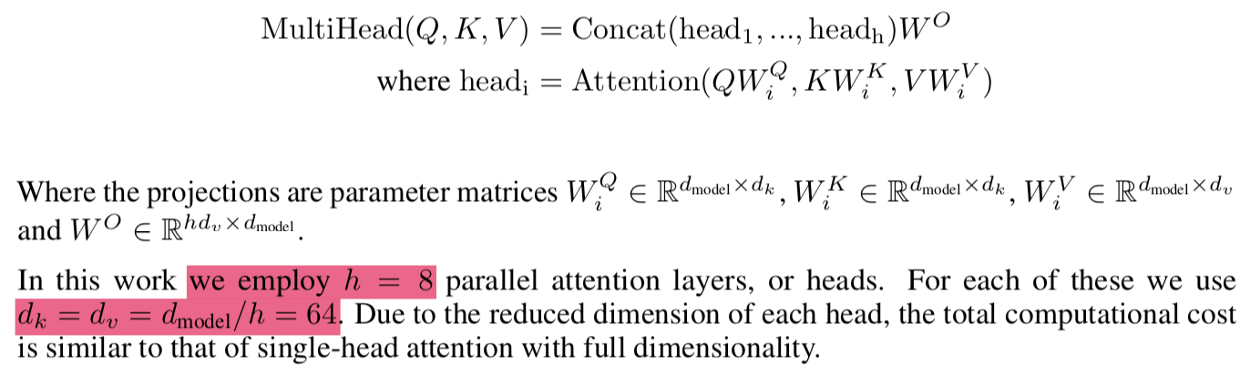
3.2.2. Multi-Head Attention
- Single Attention function을 $d_{model}$차원의 keys, values, queries에 적용하기보다 다른 $d_{k}$, $d_{k}$, $d_{v}$차원을 갖는 queries, keys, values에 h times 적용하는 것이 더 좋다는걸 알게됨
- 한 마디로하면, 그냥 한번만 Attention function쓰는게 아니라, 기존 Dim을 쪼개서 여러개로 나누고 거기에 여러번 Attention funcion 적용하면 더 다양한 Attention이 적용되고(여기엔 살짝 랜덤한..부분이 있겠지) 더 다양한 representation을 얻을 수 있게 된다는 말임
- 차원을 나눈 상태에서 Attention function은 병렬적으로 계산되고 $d_v$ 차원의 output vectors가 생성됨
 {: height=”50%” width=”50%”}
- Q, K, V는 문장 내에서 sequence정보를 포함하고 있는 Notation인듯
- dim of Q == num of tokens X $d_{model}$ 로 생각하면 될 듯
- 본 논문에서는 mutli-head를 8개로 나눠서, 전체 512 차원을 64 차원의 8개 유닛으로 만듬
- 원래는 input 임베딩을 쪼개고, 거기에 맞는 fc를 넣어주면 된다고 생각했는데, $W_{i}^Q$를 $Q$에 곱해 주는거 자체가 input 임베딩을 쪼개는 것임 결과 차원이 num of toknes X $d_{k}$로 나오니까
1 | def split_head(self, vector): |
3.2.3. Applications of Attention in our Model
- 트랜스포머에서는 멀티헤드 어텐션을 3곳에 적용함
- 첫번째, “encoder-decoder Attention” layer 에 적용함
- decoder의 input에 대해서 Attention 적용하고 그 결과를 Query로 만든 다음 레이어에 적용할때 encoder의 output을 key,value로 사용함
- 이렇게 하면 decoder의 input도 모두 고려하면서, encoder의 output도 모두 고려하는 seq2seq 모델에 attention을 적용한것과 비슷하게 됨
- 두번째, “self-attention layer” in encoder 에 적용함, 이 역시도 sequence 내의 모든 position을 다 고려할 수 있음
- 세번째, “self-attention layer” in decoder 에 적용함, 보지못한 정보를 보는 것을 막기 위해 (
to prevent leftward information flow in the decoder to preserve the auto-regressive property) scaled dot-product attention안에 마스킹을 적용함(minus infinity) (Figure 2)
1 | def create_padding_mask(seq): |
3.3. Position-wise Feed-Forward Networks
- Attention sub-layers 다음엔 FC(Fully connected feed-forward network)가 붙게 됨
- two linear transformation with ReLU가 적용됨
 {: height=”50%” width=”50%”}
 - input and output dim, $dim_{model}$ = 512
- inner-layer dim, $dim_{ff}$ = 2048
3.4. Embeddings and Softmax
- 다른 sequence transduction model과 같이 여기서도 $d_{model}$ 차원을 갖는 learned embeddings을 사용함
- learned linear transformation & softmax function을 사용함
- two embedding layers, pre-softmax linear transformation에 대해서 weight matrix를 공유함
- embedding layer에서 weights에 $\sqrt{d_{model}}$를 곱해줌 (스케일링)
1 | x = self.embed(inputs) # (batch, seq, word_embedding_dim) |
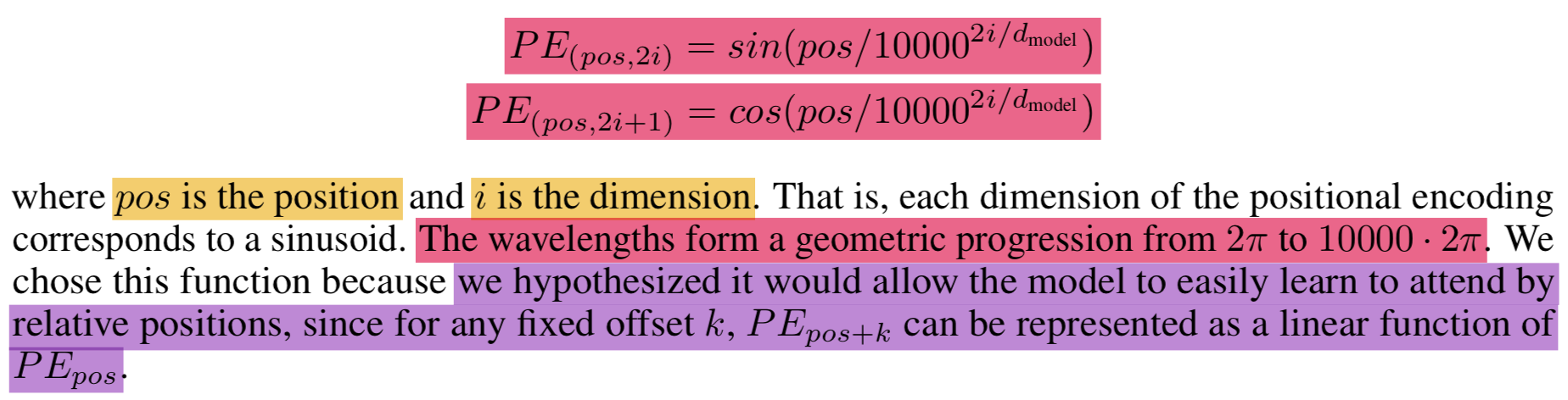
3.5. Positional Encoding
- 본 모델에서는 recurrence도 convolution도 없기 때문에 position 정보를 알 수가 없음
- 그렇기 때문에 position information을 inject해줘야함
- “positional encodings”를 input embedding에 더하겠음 (
input embedding + positional encodings)
 {: height=”50%” width=”50%”}
1 | def add_positional_encoding(self, embed): |
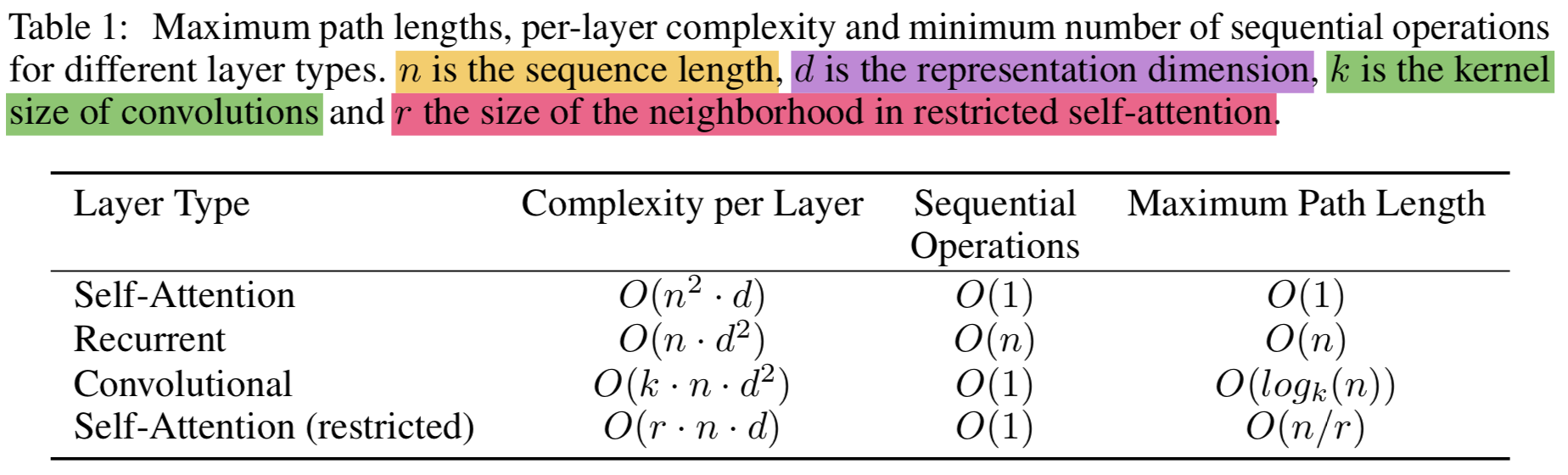
4. Why Self-Attention
- self-attention과 다른 알고리즘 비교하겠음
- 대부분은 Self-Attention이 좋음 Complexity빼고! 이 부분은 주변의 r개만 보는 restricted self-attention 버전으로 해결할수 있을듯
 {: height=”50%” width=”50%”}
5. Training
5.1. Training Data and Batching
- Data1: WMT 2014 English-German dataset
- 4.5 million sentence pairs
- byte-pair encoding
- source-target vocabulary of about 37,000 tokens
- Data2: larger WMT 2014 English-French dataset
- 36M sentences
- split tokens in a 32,000 word-piece vocabulary
- sentence length가 비슷한 애들끼리 batch 처리함
- 각 배치당 25,000 source tokens, 25,000 target tokens 정도를 포함함
5.2. Hardware and Schedule
- 8 NVIDIA P100 GPUs 사용
- base model
- each training step은 0.4 초 걸림
- 학습에 사용한 steps or time: 100,000 steps or 12 hours
- big models
- 스텝당 1.0 초 걸림, 300,000steps (3.5 days) 소요
5.3. Optimizer
- Adam
- $\beta_1 = 0.9$, $\beta_2 = 0.98$, $\epsilon = 10{^-9}$
- learning rate 바꿔줌
- warmup_steps 에서는 lr이 linearly 증가함
- 그 후에는 inverse square root of the step number 비율로 감소함
- warmup_steps = 4,000으로 셋팅함
 {: height=”50%” width=”50%”}
5.4. Regularization
- 3가지 기법 적용함 (
왜 논문에는 근데 레벨이 2개밖에 없지..)- Residual Dropout
- 각 sub-layer의 output에 미리 적용해서 나중에 sub-layer input에 더해주고 정규화함
- input embedding과 positional embedding을 더한 결과에 대해서도 적용함 (encoder & decoder 모두)
- $P_{drop} = 0.1$
- Label Smoothing
- label smoothing 적용함 $\epsilon_{ls} = 0.1$
- This hurts perplexity, as the model learns to be more unsure
- 하지만 Accuracy와 BLEU scroe는 올라감
- 출처: [36] Christian Szegedy, Vincent Vanhoucke, Sergey Ioffe, Jonathon Shlens, and Zbigniew Wojna. Rethinking the inception architecture for computer vision. CoRR, abs/1512.00567, 2015.
- Residual Dropout
6. Results
6.1. Machine Translation
- Beam search 적용함
- beam size = 4
- length penalty $\alpha = 0.6$
- Hyper params는 Development set 기준으로 실험적으로 선택함
- Maximum output length = input length + 50
 {: height=”50%” width=”50%”}
6.2. Model Variations
- 모델 컴포넌트들의 중요도를 평가하기 위해 varied model에 대해서 평가함
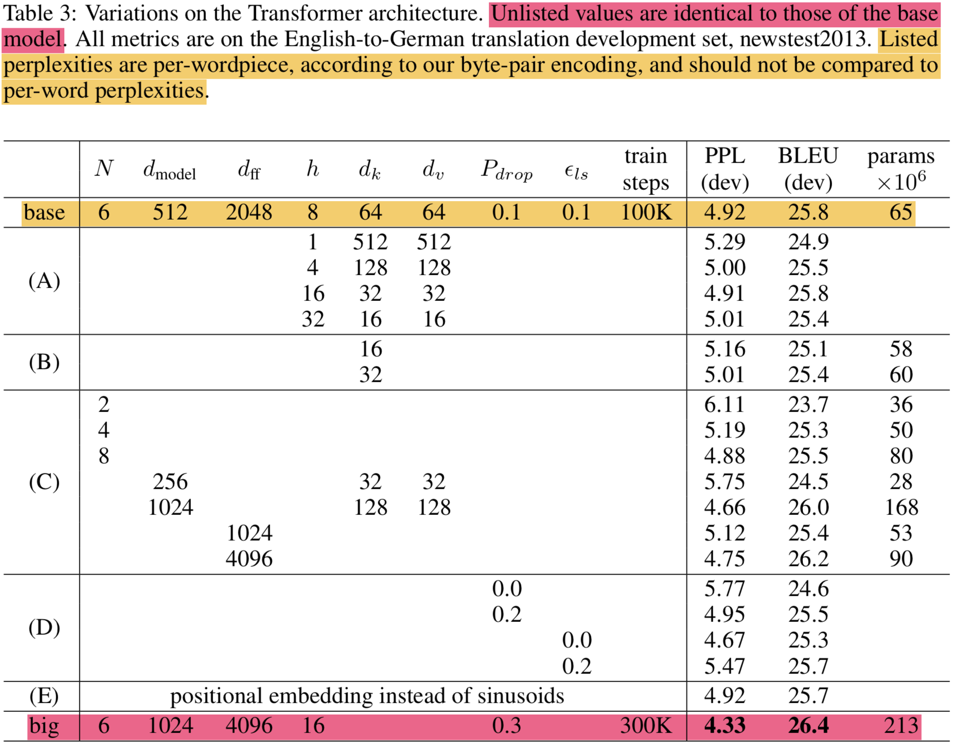 {: height=”50%” width=”50%”}
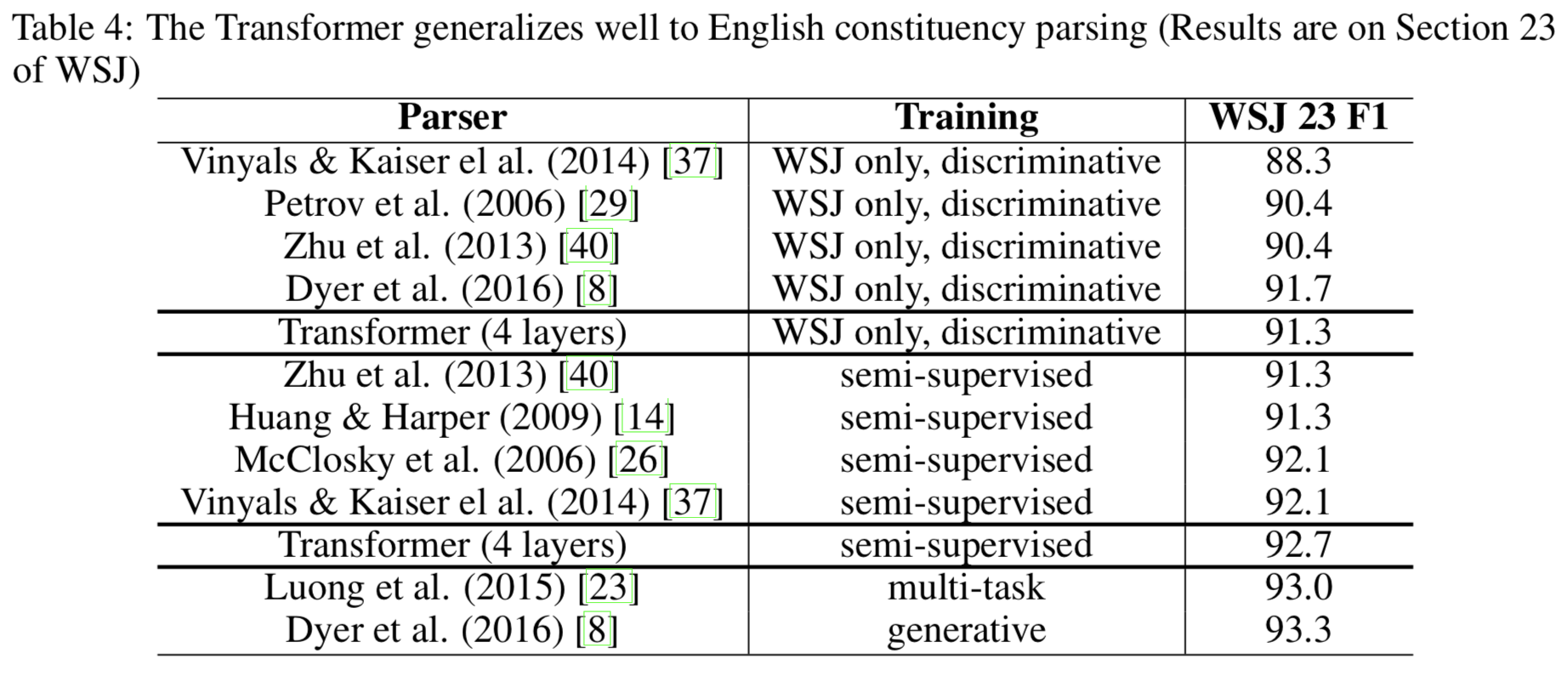
6.3. English Constituency Parsing
- Transformer가 generalize 잘 되는지 평가함
- 생각보다 잘 됨
 {: height=”50%” width=”50%”}
7. Conclusion
- Attention만 의존하는 모델 처음으로 발표함
- recurrent layer를 multi-headed self-attention을 쓰는 encoder-decoder 구조로 대체함
- rnn, cnn보다 학습 빨리됨
- NMT에서 SOTA 찍음
- 다른 도메인에도 적용 될수 있을거라 생각함
Acknowledgements
- ByteNet저자였던 Nal Kalchbrenner와, Stephan Gouws의 comments, corrections and inspiration에 감사함
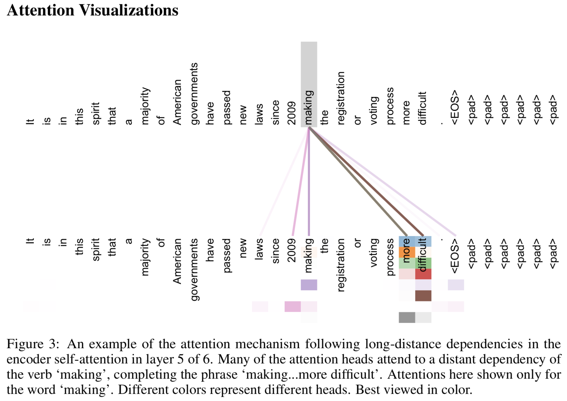
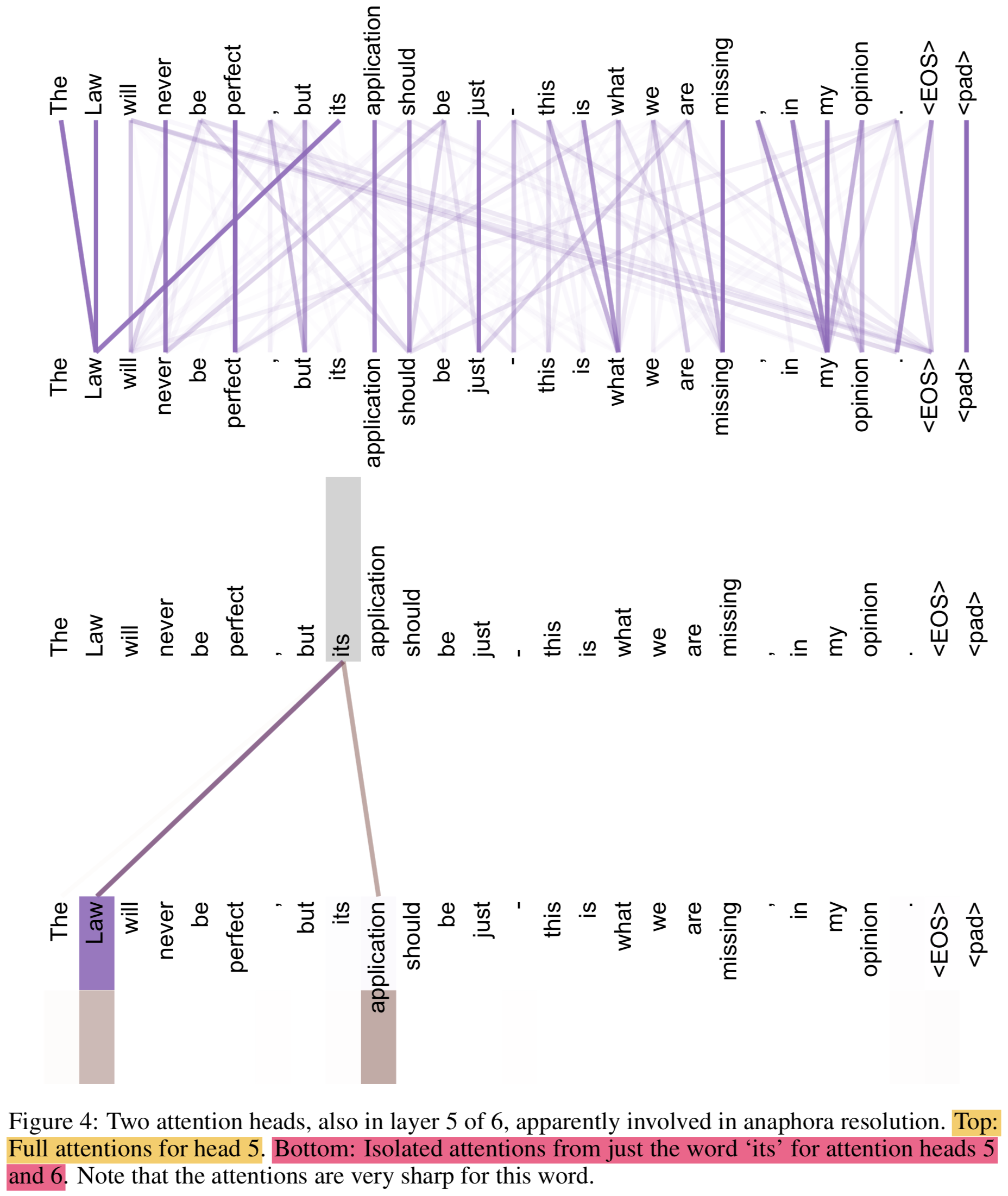
Attention 시각화
 {: height=”50%” width=”50%”}
 {: height=”50%” width=”50%”}
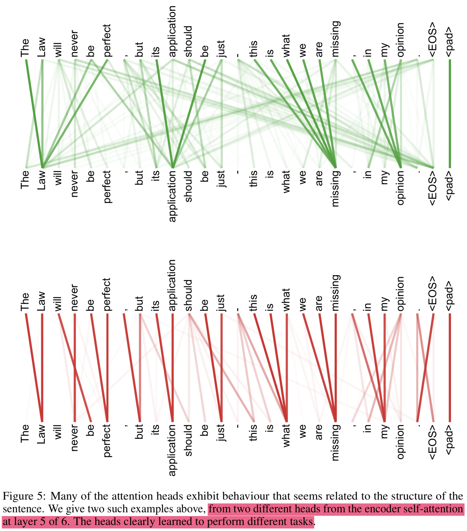 {: height=”50%” width=”50%”}
Attention Is All You Need
https://eagle705.github.io/2019-05-01-Attention_is_All_you_need/