Stochastic Answer Networks for Natural Language Inference (SAN)

Author

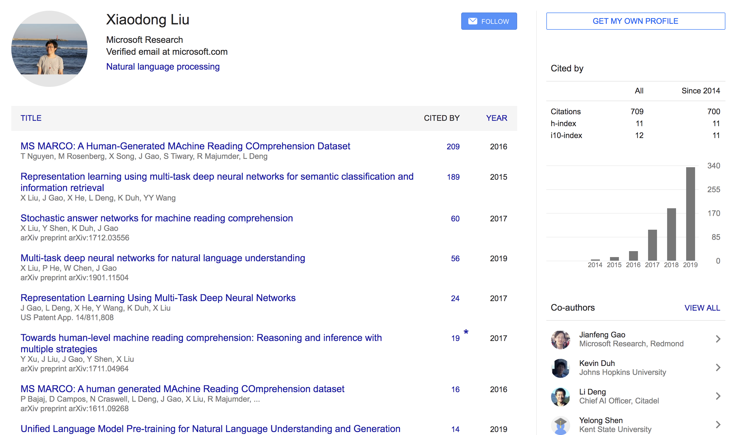
• 저자:Xiaodong Liu†, Kevin Duh and Jianfeng Gao (Microsoft Research, Johns Hopkins University)

Who is an Author?

Xiaodong Liu 라는 친구인데 꽤 꾸준히 연구활동을 하는 친구인것 같다.

{: height=”50%” width=”50%”}

느낀점

• turn의 정보를 반영하기에 attention은 필수
• 하지만 5턴 이상 반영하는건 쉬운게 아님(여기서도 10개까지 했지만 5~6개가 best라고 했음)
• multi turn을 위한 architecture를 pretrained model를 feature extractor로 써서 결합해서 쓰는게 앞으로의 연구 트렌드가 될 듯

Abstract

• multi-step 에서 inference를 좀 더 잘하게 해주기 위한 방법을 연구함
• 그냥 주어진 input에 대해서만 쓰는게 아니라 state를 저장하면서 iteratively refine하면 모델이 잠재적으로 더 복잡한 inference도 가능하게 만들어줄 것임
• SNLI, MultiNLI, SciTail, Quora Question Pairs 데이터셋에서 SOTA를 기록함

1. Motivation (intro가 아니라 Motivation이네 특이하군..)

• NLI, 다른말로 Recognizing textual entailment (RTE)로 알려진 태스크는 sentence pair의 관계를 추론하는 것임 (e.g. premise and hypothesis)
• 이게 왜 어렵냐면 문장의 의미를 완벽히 이해해야 하기 때문임 (문법적, 요소적인 의미 둘다)
• 예를들어, MultiNLI dataset 같은 경우엔 premise와 hypothesis간의 정보들에 대해서 multi-step synthesis가 필요함
• 여러가지 선행 연구들에 따라서 multi-step inference strategies on NLI에 대해 조사해보고자함

2. Multi-step inference with SAN

{: height=”50%” width=”50%”}

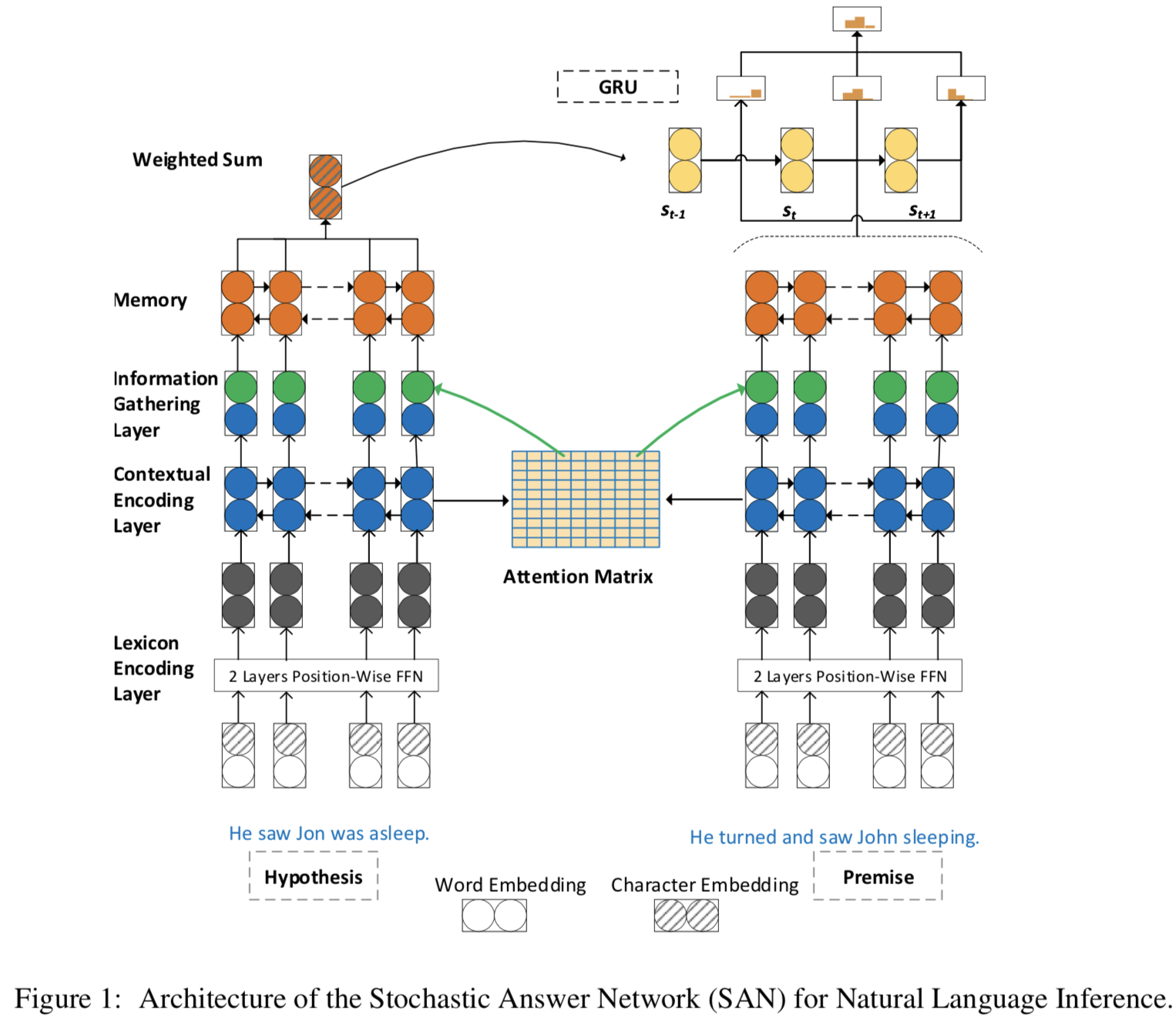
• NLI task는 P, H의 관계 R을 찾는게 목표임
• 관계 R은 entailment, neutral and contradiction 이거 3개로 이루어짐 (연관, 중립, 모순)
• 기존 single-step에서는 $f(P, H) \rightarrow R$ 를 만족하는 f를 학습하는게 목표였지만, multi-step에서는 여기에 recurrent state $s_t$ 를 추가하고 이것을 업데이트해서 사용함
• 제안하는 모델은 기존 MRC multi-step inference literature를 착안함
• 본 모델에서는 4가지 레이어가 있음

Lexicon encoding layer:

• computes word representations
• word embedding이랑 char embedding을 concat 해서 OOV 해결
• word랑 char에 대해 각각 position-wise feedforward network 태워서 계산함
• outputs: $ E^{p} \in \mathbb{R}^{d \times m} \text { and } E^{h} \in \mathbb{R}^{d \times n} $
• notation: premise가 m개의 토큰, hypothesis가 n개의 토큰임, d는 hidden size

Contextual encoding layer:

• modifies these representations in context
• maxout layer 사용했고, BiLSTM 썼는데 두 방향에 대해서 concat해서 썼음
• outputs: $ C^{p} \in \mathbb{R}^{2 d \times m} $, $ C^{h} \in \mathbb{R}^{2 d \times n} $

Memory generation layer:

• gathers all informa- tion from the premise and hypothesis and forms a “working memory” for the final answer module
• Attention Mechanism으로 working memory 구성함
• P와 H에 있는 토큰들의 유사성을 측정하기 위해 dot product attention을 사용함
• 보통 쓰는 scalar norm을 쓰지 않고, Layer projection 해서 사용함. 그래서 notation에 hat이 붙은 것임
• $ A=d r o p o u t\left(f_{a t t e n t i o n}\left(\hat{C}^{p}, \hat{C}^{h}\right)\right) \in \mathbb{R}^{m \times n} $
• A를 attention matrix라 칭함, dropout 적용되어있음

Information Gathering Layer:

• premise와 hypothesis의 모든 정보를 모아서 다음과 같이 나타냄
• $ U^{p}=\left[C^{p} ; C^{h} A\right] \in \mathbb{R}^{4 d \times m} $
• $ U^{h}=\left[C^{h} ; C^{p} A^{\prime}\right] \in \mathbb{R}^{4 d \times n} $
• notation:
• ; 은 concatenation을 의미함
• ′은 transpose를 의미함
• outputs: $ \begin{array}{l}{ M^{p}=\operatorname{BiLSTM}\left(\left[U^{p} ; C^{p}\right]\right) \text { and } M^{h}=} {\operatorname{BiLSTM}\left(\left[U^{h} ; C^{h}\right]\right)}\end{array} $

Final answer module:

• predicts the relation between the premise and hypothesis. compute over T memory steps and output the relation label.
• states와 이전 메모리에 대한 weighted sum값인 x를 feature화 해서 그 스텝에서의 $ P_{t}^r $(확률) 값을 구하고, 실제 inference할땐 이전 스텝의 모든 $ P_{t}^r $ 에 대해 평균 취해서 구함
• inintial state $ s_{0} $
• $ M^{h}: s_{0}=\sum_{j} \alpha_{j} M_{j}^{h} $
• $ \alpha_{j}=\frac{\exp \left(\theta_{2} \cdot M_{j}^{h}\right)}{\sum_{j^{\prime}} \exp \left(\theta_{2} \cdot M_{j^{\prime}}^{h}\right)} $
• time step t는 {1, 2, …, T - 1} 까지임
• $ s_{t}=G R U\left(s_{t-1}, x_{t}\right) $
• $ x_{t}=\sum_{j} \beta_{j} M_{j}^{p} \text { and } \beta_{j}=\operatorname{softmax}\left(s_{t-1} \theta_{3} M^{p}\right) $
• 정리하면 initial state는 h에서 꺼내옴
• state $ s_t $는 GRU에 이전 state와 $ x_t $ 값을 태워서 만들어내는데, $ x_t $는 premise의 메모리들에 대한 weighted sum 값임. 결국 이전 states와 메모리에 대한 weighted sum 값을 보겠다는 것임
• 이 weighted sum은 이전 state ($ s_{t-1} $)와 현재 메모리에 $ \theta_3 $ param을 곱해서 만든 값에 softmax를 한 것임 (여기서 어떻게 다른 값들이 나와서 softmax 를 할 수 있는건지 고민이 되는데, time step에 대한 메모리가 아니라 전체에 대한 메모리 값에 대해서 연산해서 그런듯)
• t step에 대한 결과 값은 이러한 states와 x값(메모리에 대한 weighted sum) 들을 feature화 해서 softmax 씌움
• t step outputs: $
  P_{t}^{r}=\operatorname{softmax}\left(\theta_{4}\left[s_{t} ; x_{t} ;\left|s_{t}-x_{t}\right| ; s_{t} \cdot x_{t}\right]\right)
  $
  • $\theta_{4}$가 class로 맵핑시켜주는 param일듯..!
  • Each $ P_{t}^{r} $ is a probability distribution over all the relations
• final output: $
  P^{r}=\operatorname{avg}\left(\left[P_{0}^{r}, P_{1}^{r}, \ldots, P_{T-1}^{r}\right]\right)
  $

stochastic prediction dropout

• 학습 도중에 stochastic prediction dropout이라는 기법을 적용함 (avg ops 전에 적용!)
  • Decoding 때 all outputs에 대해 avg해서 robustness를 개선함
  • 보통의 dropout at the final layer level은 다음과 같은 문제가 있음
    • Dropout at the final layer level, where ran- domness is introduced to the averaging of predic- tions, prevents our model from relying exclusively on a particular step to generate correct output
  • 새로 적용한 기법은 intermediate node-level에 dropout을 적용함 (이게 무슨뜻일까)

3. Expriments

3.1 Dataset

SNLI

• MultiNLI
• Quora
• SciTail

3.2 Implementation details

• The spaCy tool2 is used to tokenize all the dataset
• PyTorch is used to implement our models
• word embedding with 300-dimensional GloVe word vectors
• character encoding, we use a concatenation of the multi-filter Convolutional Neural Nets with windows 1, 3, 5 and the hidden size 50, 100, 150
• lexicon embeddings are d=600-dimensions
• The hidden size of LSTM in the contextual encod- ing layer, memory generation layer is set to 128
  • the input size of output layer is 1024 (128 * 2 * 4) as Eq 2
• The projection size in the atten- tion layer is set to 256
• Training
  • weight normalization
  • dropout rate is 0.2
  • mini-batch size is set to 32
  • Our optimizer is Adamax
  • learning rate is initialized as 0.002 and decreased by 0.5 after each 10 epochs

3.3 Results

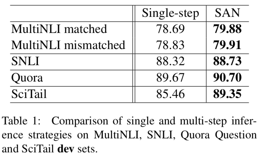
• Single-step과 multi-step (SAN) 비교
• multi-step 비교한 모델이 더 잘함
  {: height=”50%” width=”50%”}
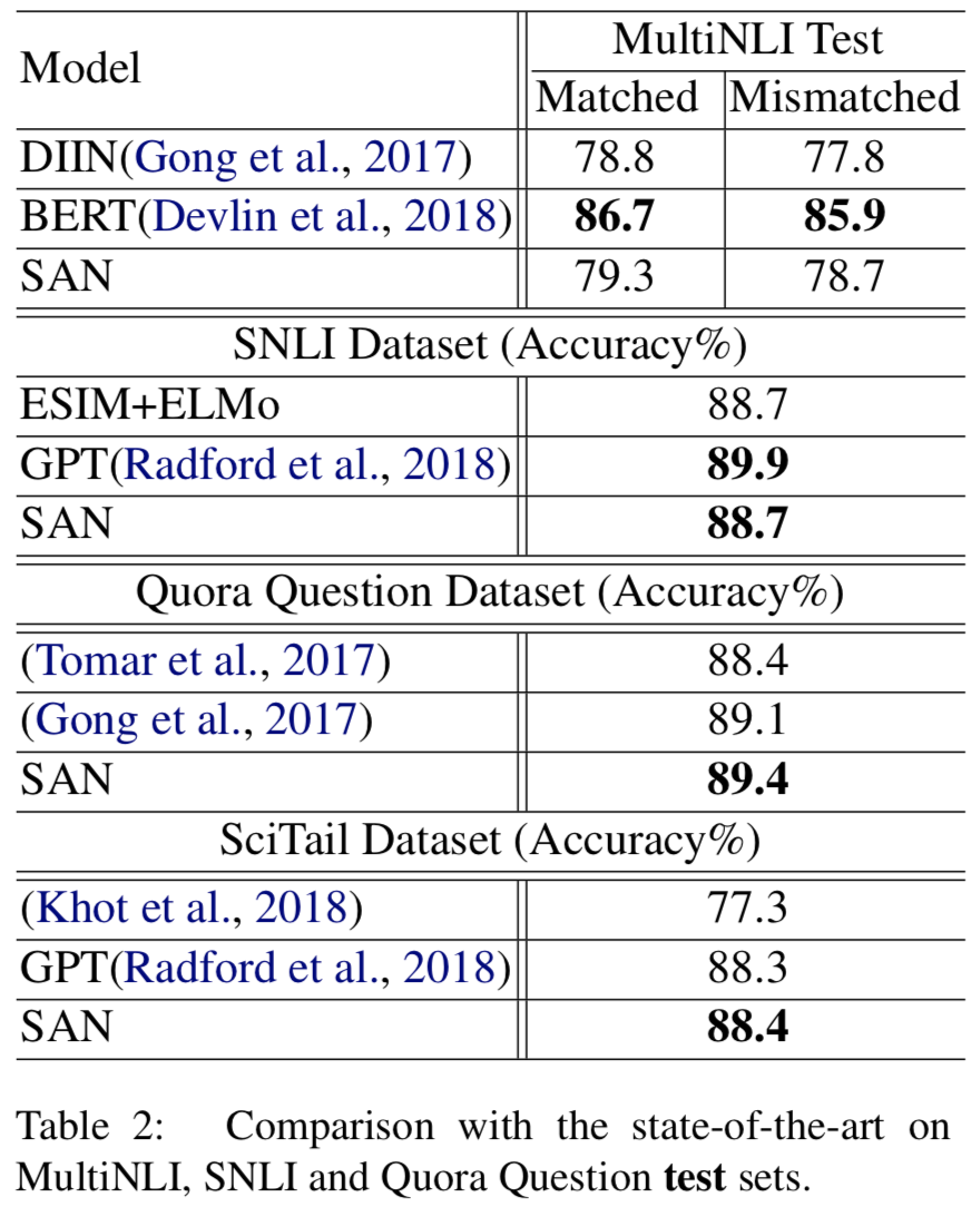
• 대부분 잘나왔고 BERT랑 GPT에 좀 밀리는 감이 있지만 적은 파라미터로 잘했다고 저자는 어필함
• BERT위에 SAN answer module 얹어서 해봤는데 잘나옴
• infernece step은 2보다 5, 6등이 더 잘나옴.. 실험에서는 5로 fix하고 실험함
  {: height=”50%” width=”50%”}

4. Conclusion

• multi-step infernece를 위한 방법을 탐색해봄
• stochastic answer network (SAN)라는 이름으로 제안함
• 몇몇 task에서 SOTA 찍음
• 다음엔 pretrained contextual embedding (ELMo)와 함께 써보거나 GPT내의 multi-task learning중 하나로 적용해볼 생각임

Reference

• Latex Symbols
• Latex generation tools